In this post we will be looking at the Transformer architecture in detail. You can also find the code for this post on my GitHub Repository.

ATTENTION: All the images are taken from Natural Language Processing with Transformers, Revised Edition book.

Transformer Anatomy

Transformers represent a groundbreaking paradigm shift in artificial intelligence and natural language processing. The original transformer is based on the encoder-decoder architecture that is used for different tasks such as machine translation, named entity recognition, text summarization and suchlike.

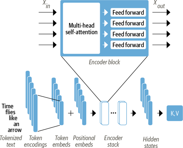
Encoder

The encoder consists of many encoder stacked next to each other. The encoder converts an input sequence of tokens into a sequence of embedding vecotrs, so called hidden state or context. Each encoder layer recieves a sequence of embeddings and feed them through the following sublayers see Figure 2:

• A multi-head attention layer
• A fully connected feed-forward layer that is applied to each input embedding

Decoder

Use the encoder’s hidden states to iteratively generate an output sequence of tokens, one token at a time.

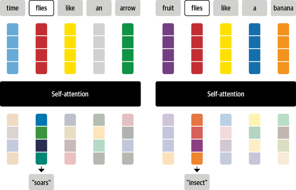
Self-Attention

The attention is a mehcanism that allows neural networks to assign a different weight to each token in the sequence. The main idea behind the self-attention is that instead of using a fixed-embedding for each token, we can use the whole sequence to compute a weighted-average of each embedding. Given a sequence of token embeddings $x_1, x_2, …, x_n$ self-attention produces a sequence of new embeddings $x’_1, x’_2, …, x’_n$ where each $x’_i$ is a linear combination of all the $x_j$:

The coefficients $w_{ij}$, referred to as attention weights, play a pivotal role in self-attention mechanisms. To grasp the concept of self-attention, consider the word “flies.” Initially, one might associate it with the small insects. However, with additional context such as “time flies like an arrow,” a new understanding emerges, revealing that “flies” functions as a verb. Through the efficacy of self-attention, we can assign greater weights $w_{ij}$ to the embeddings of tokens “time” and “arrow,” effectively incorporating the context. This allows the model to prioritize relevant information, demonstrating the power of self-attention in capturing intricate relationships within the sequences. A diagram of process is show in Figure 3.

Attention Weights Calculation

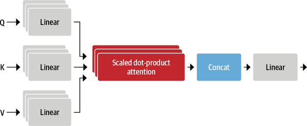
The most common way to calculate the self-attention weights is to use scaled dot-product. The following four steps are required to implement this mechanism:

• Create three vectors called query, key, value for each token embedding.
• Compute attention scores. At this stage we need to determine the similarity between the query, and key vectors. The similarity function which is used here is the dot-product. Queries and keys that are similar will have a large dot product, while those with lower similarity will have less or zero dot product. The output from this step is called the attention scores and for a sequence of $n$ tokens we will have a matrix of $n \times n$ as attention score matrix.
• Compute attention weights by scaling and normalizing dot products. At this step we apply a scaling factor to stabilize training by normalizing variance. Afterwards, they will be normalized with a softmax to ensure all the column values sum to 1. The resulting $n \times n$ matrix now contains all the attention weights, $w_{ji}$.
• Update the token embeddings. Once the attention weights are cmputed, we multiply them by the value vector $v_1, v_2, …, v_n$ to update the representation for embedding $x’_i = \sum w{ji} v_j$. The whole process is shown in Figure 4.

Multi-headed Attention

The self-attention applies three different linear transformations to each embedding to generate the query, key and value vectors. In other words, it projects them into three different spaces containing their own set of learnable parameters. This process allows the self-attention layer to focus on different semantic aspects of the sequence. Each of these linear projections called attention head. The resulting multi-head attention layer is shown in Figure 5.

The reason for having more than one heads is to allow the model focusing on several aspects at once. For instance, one head can focus on subject-verb interaction, while the other finds nearby adjectives.

The implementation of a single attention head:

class AttentionHead(nn.Module):
    def __init__(self, embed_dim, head_dim): # if we have 12 heads then head_dim = embed_dim/12. For instance, if embed_dim = 768 then head_dim = 64
        super().__init__()
        self.q = nn.Linear(embed_dim, head_dim)
        self.k = nn.Linear(embed_dim, head_dim)
        self.v = nn.Linear(embed_dim, head_dim)
        
    def forward(self, hidden_state):
        attn_outputs = scaled_dot_product_attention(self.q(hidden_state), self.k(hidden_state), self.v(hidden_state))
        return attn_outputs

Now we will create the Multi-Head Attention layer by concatenating the outputs of all the attention heads:

class MultiheadAttention(nn.Module):
    def __init__(self, config):
        super().__init__()
        num_heads = config.num_attention_heads
        embed_dim = config.hidden_size
        head_dim = embed_dim // num_heads
        self.attention_heads = nn.ModuleList([AttentionHead(embed_dim, head_dim) for _ in range(num_heads)])
        self.linear = nn.Linear(embed_dim, embed_dim) # This is the linear layer that will be applied to the concatenated outputs of all the attention heads ->
            # to produce an output tensor shape of [batch_size, seq_len, embed_dim]
        
    def forward(self, hidden_state):
        attention_outputs = torch.cat([attn_head(hidden_state) for attn_head in self.attention_heads], dim=-1) # dim=-1 means we are concatenating along the last dimension 
        multihead_attention_outputs = self.linear(attention_outputs)
        return multihead_attention_outputs

Now it is the turn to discuss the last piece of encoder which is position-wise feed forward network.

The Feed-Forward Layer

The feed-forward sublayer in both the encoder and decoder consists of a straightforward two-layer fully connected neural network. An distinctive characteristic of this sublayer is its ability to process each embedding independently, as opposed to processing the entire sequence of embeddings as a single vector. A rule of thumb from the literature is for the hidden size of the first layer to be four times the size of the embedding and a GELU activation function is most commonly used. The implementation for the feed-forward layer:

class Feedforward(nn.Module):
    def __init__(self, config):
        super().__init__()
        self.linear1 = nn.Linear(config.hidden_size, config.intermediate_size)
        self.linear2 = nn.Linear(config.intermediate_size, config.hidden_size)
        self.gelu = nn.GELU()
        self.dropout = nn.Dropout(config.hidden_dropout_prob)
        
    def forward(self, hidden_state):
        ff_outputs = self.dropout(self.linear2(self.gelu(self.linear1(hidden_state))))
        return ff_outputs

We now have all the components to create a transformer encoder layer. The only thing that we have to check is that where we can put the skip connections and layer normalization.

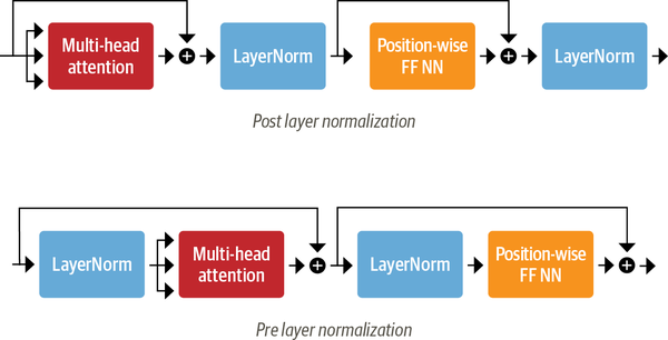
Adding Layer Normalization

The Transformer architecture employs layer normalization and skip connections. Layer normalization ensures zero mean and unity variance for each batch input, while skip connections pass a tensor to the next layer without processing, adding it to the processed tensor. In deciding where to place layer normalization within Transformer’s encoder or decoder layers, two main choices are commonly found in the literature:

• Post layer normalization: The Transformer paper places layer normalization between skip connections, a setup challenging to train from scratch due to potential gradient divergence. To mitigate this, a common practice is learning rate warm-up, gradually increasing the rate from a small value to a maximum during training.
• Pre layer normalization: this is the most common used architecture. it places the layer normalization within the span of the skip connections. The difference between these two architectures is indicated in Figure 6

Now we can implement the encoder layer:

class TransformerEncoderLayer(nn.Module):
    def __init__(self, config):
        super().__init__()
        self.attention = MultiheadAttention(config)
        self.feedforward = Feedforward(config)
        self.layernorm1 = nn.LayerNorm(config.hidden_size)
        self.layernorm2 = nn.LayerNorm(config.hidden_size)
        
    def forward(self, x):
        #  Apply layer normalization and then copy input into query, key, value
        hidden_state = self.layernorm1(x)
        
        # Apply multi-head attention with a skip connection 
        x = x + self.attention(hidden_state)
        # Apply feed forward layer with a skip connection
        x = x + self.feedforward(self.layernorm2(x))
        return x

Since the multi-head attention layer is effectively a fancy weighted sum, the information on token position is lost and we have to add the positional embeddings.

Finally, it is the time to pull everything together and implement the full transformer encoder combining embeddings with the encoder layer:

class TransformerEncoder(nn.Module):
    def __init__(self, config):
        super().__init__()
        self.embeddings = nn.Embedding(config)
        self.encoder_layers = nn.ModuleList([TransformerEncoderLayer(config) for _ in range(config.num_hidden_layers)])
        
    def forward(self, x):
        hidden_state = self.embeddings(x)
        for encoder_layer in self.encoder_layers:
            hidden_state = encoder_layer(hidden_state)
        return hidden_state

Adding a Classification Head

Transformer models usually have two main parts: 1. Task-independent body, and 2. task-specific head. What we have implemented so far is the task-independent body. As a result, we have to attach a classification head to this body. We have a hidden state for each token, but we only need to make one prediction as the predicted next token. Traditionally, the first token ([CLS]) is used for the prediction and we can attach a dropout and a linear layer to make a classification prediction. Let’s implement it:

 class TransformerForSequenceClassification(nn.Model):
    def __init__(self, config):
        super().__init__()
        # We will use the transformer encoder to encode the input sequence
        self.encoder = TransformerEncoder(config)
        # We will use the hidden state of the first token of the sequence to make the classification
        self.classifier = nn.Linear(config.hidden_size, config.num_labels)
        
    def forward(self, x):
        x = self.encoder(x)
        x = x[:, 0, :] # We take the first token of the sequence
        logits = self.classifier(x)
        return logits

Decoder

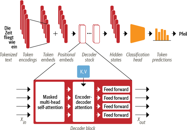
As depicted in Figure 7, the main difference between the decoder and encoder is that the decoder has two attention sublayers:

• Masked multi-head self-attention layer: This sublayer is to ensure that the decoder does not cheat during training copying the target tokens. We mask the input to make sure that at each timestep the model predicts only based on the past outputs.
• Encoder-decoder attention layer: This sublayer performs multi-head attention over the output key and value vectors of the encoder stack, with the intermediate representations of the doceder acting as the queries. This is advantegous in the manner learning how to relate tokens from two different sequences, such as two different languages.